Quick Start Guide

Hello, world!

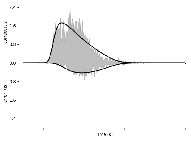
To get started, let’s simulate a basic model and plot it. For simplicity, we will use all of the model defaults: a drift rate of 0, a noise standard deviation of 1, a bound of 1, a starting point in the middle of the bounds, a non-decision time of 0, and a uniform mixture model. (More on each of these later.)

import matplotlib.pyplot as plt
import pyddm
m = pyddm.gddm()
s = m.solve()
plt.plot(s.t_domain, s.pdf("correct"))
plt.show()

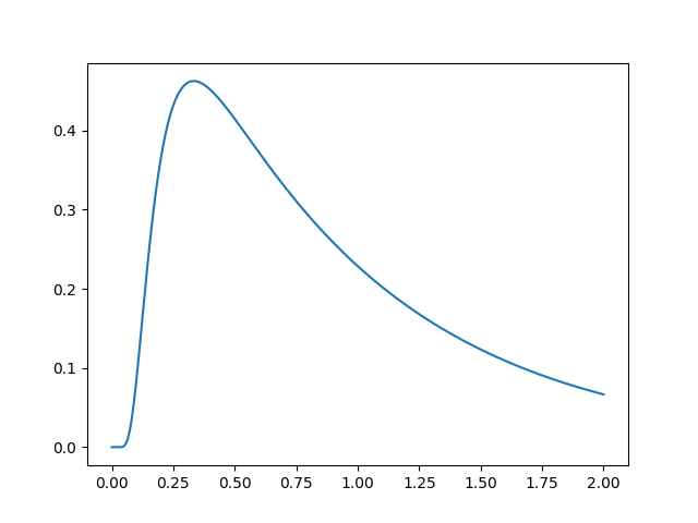
Congratulations! You’ve successfully simulated your first model! Let’s dig in a bit so that we can define more useful models.

For the rest of this tutorial, we will slowly build a generalized drift diffusion model (GDDM), validate the model, and then fit the model to an open dataset. As we do, we will illustrate the main concepts of PyDDM to so you can start building your own models.

Download this full example

Note

There are two ways to build models with PyDDM: the classic object-oriented interface, and the gddm() function. Here, we will discuss the gddm() function: it supports almost all of the features of the object-oriented interface, but is much easier to use. Once you have finished this tutorial, if you are interested in the object-oriented interface, you can access the Object-oriented interface tutorial.

A model with fixed parameters

First, let’s see how we can modify the different pieces of the model given above. For consistency, we will refer to these pieces (drift, noise, bound, starting position, non-decision time, and mixture coefficient) as “components”. All components will be defined within the gddm() function. The components available in the gddm() function are:

• drift: the drift rate, i.e., the amount of evidence that would be accumulated in 1 sec if there was no noise.

• noise: the noise level, i.e., the standard deviation of noise. By tradition, this is frequently set to 0.1 or 1.0. If not specified, it defaults to 1.0.

• bound: the height of the boundary on each side. (So, the total separation of the boundaries will be twice this value.)

• starting_position: the initial position of the diffusion process. A value of 1 indicates a starting position on the upper boundary, -1 on the bottom boundary, and 0 in between. (This differs from some other packages, which define 0 as the lower boundary and 1 as the upper boundary.)

• nondecision: the non-decision time, in units of seconds. Both positive and negative values are valid (though usually you will want it to be positive).

• mixture_coef: By default, PyDDM returns an RT distribution which is a mixture model of the GDDM RT distribution and the uniform distribution. This parameter defines the ratio of uniform distribution to GDDM RT distribution. Set to 0 to disable the mixture model. By default, this is 0.02. (Mixture models assist with model fitting when using maximum likelihood, which we will discuss later in this tutorial.)

So, for a model with a drift rate of 0.5, a noise level of 1.0, a bound height of 0.6, a starting position of 0.3 (slightly biased towards the upper bound), and a non-decision time of 0.2 sec, the model would be:

model = pyddm.gddm(drift=0.5, noise=1.0, bound=0.6, starting_position=0.3, nondecision=0.2)

We can show information about our model using the show() function:

model.show()

which displays:

Model information:
Choices: 'correct' (upper boundary), 'error' (lower boundary)
Drift component DriftConstant:
    constant
    Fixed parameters:
    - drift: 0.500000
Noise component NoiseConstant:
    constant
    Fixed parameters:
    - noise: 1.000000
Bound component BoundConstant:
    constant
    Fixed parameters:
    - B: 0.600000
IC component ICPointRatio:
    An arbitrary starting point expressed as a proportion of the distance between the bounds.
    Fixed parameters:
    - x0: 0.300000
Overlay component OverlayChain:
    Overlay component OverlayNonDecision:
        Add a non-decision by shifting the histogram
        Fixed parameters:
        - nondectime: 0.200000
    Overlay component OverlayUniformMixture:
        Uniform distribution mixture model
        Fixed parameters:
        - umixturecoef: 0.020000

Once we have a model, we can simulate or “solve” the model. Solution objects represent the probability distribution functions over time for choices associated with upper and lower bound crossings. We saw one of these, “s”, in the first example. They can also be used to generate artificial data for parameter recovery simulations. We will discuss this shortly.

sol = model.solve()

Fitting model parameters

We can also define a model with free parameters - these parameters can be fit to data, or tweaked using a GUI built into PyDDM for visualizing and modifying models. Instead of passing numbers as arguments for the different model components, we can instead pass the names of parameters to fit. Then, at the end, we use the “parameters” argument to list the parameters and their valid ranges. This argument should be a dictionary, where the key of the dictionary is the name of the parameter, and the value is a tuple containing the minimum and maximum value of the parameter. For example, if we want to fit the drift rate, the bound, and the non-decision time, but keep the noise level fixed at 1.0, we can write:

model_to_fit = pyddm.gddm(drift="d", noise=1.0, bound="B", nondecision=0.2, starting_position="x0",
                          parameters={"d": (-2,2), "B": (0.3, 2), "x0": (-.8, .8)})
model_to_fit.show()

This gives:

Model information:
Choices: 'correct' (upper boundary), 'error' (lower boundary)
Drift component DriftConstant:
    constant
    Fittable parameters:
    - drift: Fittable (default 0.196055)
Noise component NoiseConstant:
    constant
    Fixed parameters:
    - noise: 1.000000
Bound component BoundConstant:
    constant
    Fittable parameters:
    - B: Fittable (default 0.677593)
IC component ICPointRatio:
    An arbitrary starting point expressed as a proportion of the distance between the bounds.
    Fittable parameters:
    - x0: Fittable (default -0.694904)
Overlay component OverlayChain:
    Overlay component OverlayNonDecision:
        Add a non-decision by shifting the histogram
        Fixed parameters:
        - nondectime: 0.200000
    Overlay component OverlayUniformMixture:
        Uniform distribution mixture model
        Fixed parameters:
        - umixturecoef: 0.020000

Note

In the examples here, the ranges of the parameters have been chosen arbitrarily. You may have to adjust the ranges to something that works for your model and data. Usually it is better to have a range that is too large than too small, but an extremely large range will slow down fitting. Once you perform the fitting, make sure to check that your fitted parameters are not close to the minimum or maximum values you set. If they are, you may need a bigger range.

Before fitting the model, we can visualize this model using the model GUI to make sure it behaves in the way we expect. This is usually a good sanity check when constructing a new model, as well as a useful way to get an intuition of your model’s behavior.

import pyddm.plot
pyddm.plot.model_gui_jupyter(model_to_fit) # If using a Jupyter notebook
pyddm.plot.model_gui(model_to_fit) # If not using a Jupyter notebook

Note

If the model GUI does not display the controls and the simulated RT distributions, see What can I do if the model GUI doesn’t work?.

To demonstrate how to fit this model to data, let’s simulate data from the fixed-parameter model we made above. By doing so, we will perform a parameter recovery experiment. Since the models are the same except for the free parameters, we can see if fitting the free parameters to data from the fixed parameters recovers the original fixed parameters. If not, there may be something wrong with our model!

Remember the “sol” solution object we created? We will use this to simulate data. Since this contains the “solved” probability distributions from the model, we can sample from this distribution to create simulated data. Simulated data and experimental data are both captured by a “Sample” object. Later in this tutorial, we will also see how to fit free parameters to experimental data rather than simulated data.

samp_simulated = sol.sample(10000)

Now we can fit the model to the simulated data. By default, PyDDM uses differential evolution to perform the fit: it is a slower algorithm than gradient-based methods, but is much more likely to find the best fitting parameters in complex models. We use BIC as a loss function.

model_to_fit.fit(samp_simulated, lossfunction=pyddm.LossBIC, verbose=False)
model_to_fit.show()

The result of model.show() is:

Model information:
Choices: 'correct' (upper boundary), 'error' (lower boundary)
Drift component DriftConstant:
    constant
    Fitted parameters:
    - drift: 0.533938
Noise component NoiseConstant:
    constant
    Fixed parameters:
    - noise: 1.000000
Bound component BoundConstant:
    constant
    Fitted parameters:
    - B: 0.601329
IC component ICPointRatio:
    An arbitrary starting point expressed as a proportion of the distance between the bounds.
    Fitted parameters:
    - x0: 0.279759
Overlay component OverlayChain:
    Overlay component OverlayNonDecision:
        Add a non-decision by shifting the histogram
        Fixed parameters:
        - nondectime: 0.200000
    Overlay component OverlayUniformMixture:
        Uniform distribution mixture model
        Fixed parameters:
        - umixturecoef: 0.020000
Fit information:
    Loss function: BIC
    Loss function value: 5911.712503639885
    Fitting method: differential_evolution
    Solver: auto
    Other properties:
        - nparams: 3
        - samplesize: 10000
        - mess: ''

As we can see, the parameters for drift, noise, and non-decision time are close to the values from the model that generated the data. Your fitted parameters may be slightly different than the ones shown above, since there is randomness in the fitting procedure.

Note

If the model recovery fails, i.e., if the fit parameters are different than the ones you used, there are a few things to check before concluding that there as an issue with your model:

• Ensure the simulation is long enough to capture the mass of the distribution. You can do this by increasing T_dur.

• Ensure that the simulation accuracy is sufficient for your model. In practice, this means checking that dx and dt are small enough.

• Ensure you are not fitting multiple redundant parameters. For example, in the classic DDM, noise and boundary are redundant, so at least one of these parameters must be fixed.

You will learn more about these in the upcoming section Additional properties of models.

If we want to use these fitted values programmatically, we can use parameters() to obtain the fitted parameters, like:

model_to_fit.parameters()

This will return a collection of Fitted objects. These objects can be used anywhere in Python as if they are normal numbers/floats. (Actually, Fitted is a subclass of “float”!)

We can also examine different properties of the fitting process in the FitResult object. For instance, to get the value of the loss function (BIC), we can do:

model_to_fit.get_fit_result().value()

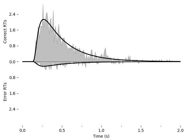
We can also draw a plot visualizing the fit. We can use one of PyDDM’s convenience methods, plot_fit_diagnostics(). We have to import pyddm.plot separately.

# Plot the model fit to the PDFs and save the file.
import pyddm.plot
import matplotlib.pyplot as plt
pyddm.plot.plot_fit_diagnostics(model=model_to_fit, sample=samp_simulated)
plt.savefig("simple-fit.png")
plt.show()

Using the Solution object sol we have access to a number of other useful functions. For instance, we can find the probability of a response using prob(), such as sol.prob("correct") for the probability of a correct response, or the entire histogram of responses using pdf(), such as sol.pdf("error") for the distribution of errors.

print(sol.prob("correct"))
print(sol.pdf("error"))

See the Solution object documentation for more such functions.

By default, the upper boundary represents correct responses and the lower boundary is error responses. We could also name the upper and lower boundary something else (e.g. “left” and “right” response), sometimes called “stimulus coding”. To do this, we need to pass the “choice_names” parameter to the Sample and the Model object. See the section on stimulus coding

Using functions as parameters

In the last section, we saw how components in PyDDM can be specified by a specific value (e.g. 0.6) or by a parameter. We did this by assigning either the value or the name of the parameter (as a string) to the component. Specifically, we wrote

model_to_fit = pyddm.gddm(drift="d", noise=1.0, bound="B", nondecision=0.2, starting_position="x0",
                          parameters={"d": (-2,2), "B": (0.3, 2), "x0": (-.8, .8)})
model_to_fit.show()

More generally, components can be defined by functions. To do this, the name of the parameter should be an argument of the function. Then, the function can be used interchangeably anywhere you would pass the name of a parameter. So, our definition is equivalent to the following definition.

model_to_fit = pyddm.gddm(drift=lambda d : d,
                          noise=1.0,
                          bound=lambda B : B,
                          nondecision=0.2,
                          starting_position=lambda x0 : x0,
                          parameters={"d": (-2,2), "B": (0.3, 2), "x0": (-.8, .8)})

Note that “lambda” is a Python feature which allows us to define short “anonymous” functions. The important thing here is that the names of the arguments are the same as the names of the parameters. We can define functions in several different ways in Python, and any of these ways will work as long as the argument is the name of the parameter. This means that the name of the function argument matters. So, for example, the following is also equivalent to the above:

def drift_function(d):
    return d
def another_func(B):
    return B
third_function = lambda x0: x0
model_to_fit = pyddm.gddm(drift=drift_function,
                          noise=1.0,
                          bound=another_func,
                          nondecision=0.2,
                          starting_position=third_function,
                          parameters={"d": (-2,2), "B": (0.3, 2), "x0": (-.8, .8)})

Functions can be useful because they allow us to specify more complex relationships among parameters. While here we have used very simple functions, any valid Python function can be used. Next, we will see additional ways that functions can be used to specify simple or complex models.

Specifying trial properties through Conditions

In most experiments, trials are not identical. Different trials may have different experimental conditions. For instance, some trials in a random dot motion task may have stronger motion coherence than others, providing different amounts of evidence that participants can use to make a decision. Or, as another example, trials may come from different blocks, where each block has different stimulus properties. In PyDDM, we refer to these differences in trials as “conditions”.

Conditions and parameters are the two primary ways we define model components in PyDDM. We previously saw how we can define components using any Python function which depends on parameters. To do this, we pass the parameters as arguments to the function. In a similar way, conditions can also be passed to these functions. So, through this, components can also depend on conditions. If we do this, we need to list all of the conditions we used at the end of the model in the argument “conditions”.

For example, suppose we have a model where the drift rate is linearly related to the stimulus coherence, or the signal strength. So, for some parameter “drift_rate_scale” and stimulus coherence condition “coh”, we have the following model:

import pyddm
m = pyddm.gddm(
    drift=lambda drift_rate_scale,coh : drift_rate_scale*coh,
    parameters={"drift_rate_scale": (-6,6)},
    conditions=["coh"])

Now, the model can only be solved if we tell the model what values to use for the conditions. When we have experimental data, conditions are loaded in with the dataset. If we want to use the model GUI without a Sample, we must tell it what conditions to use by passing in the “conditions” variable as a dictionary, where keys are the names of the conditions and values are lists of possible values for that condition. For example,

import pyddm.plot
pyddm.plot.model_gui(m, conditions={"coh": [0, .3, .6]})
pyddm.plot.model_gui_jupyter(m, conditions={"coh": [0, .3, .6]})

If we fit the model using a Sample, the Sample must have the given conditions in it. Recall that we can generate a Sample by simulating data from a Solution using the sample() function. We can’t simulate from the above model, because some parameters are not specified. So, let’s make a model where the parameter “drift_rate_scale” is fixed to 3.8 that we can use to simulate data.

m_to_sim = pyddm.gddm(drift=lambda coh : 3.8*coh, conditions=["coh"])

This model can be solved only if we specify the conditions, for example:

m_to_sim.solve(conditions={"coh": .3})

When we simulated artificial data before, our model did not depend on any conditions. If we want to add conditions to our simulated data, we must solve the model separately for each set of conditions, generate data for each separately, and then combine them together. For example,

samp_coh3 = m_to_sim.solve(conditions={"coh": .5}).sample(2000) # 2000 trials with coh=.5
samp_coh6 = m_to_sim.solve(conditions={"coh": 1.0}).sample(1000) # 1000 trials with coh=1.0
samp_coh0 = m_to_sim.solve(conditions={"coh": 0}).sample(400) # 400 trials with coh=0
sample = samp_coh3 + samp_coh6 + samp_coh0 # This preserves information about the conditions

When we fit the model, we must pass a sample object which has the appropriate conditions. If it does not, it will raise an error. Our artificial dataset now includes the “coh” condition, so we can visualize it in the model GUI without specifying the conditions if we pass the sample:

pyddm.plot.model_gui(m, sample)
pyddm.plot.model_gui_jupyter(m, sample)

Fitting will give us a value for the “drift_rate_scale” parameter, which linearly scales the condition “coh” on each trial. We can perform the fitting as before:

m.fit(sample, verbose=False)
print(m.parameters())

Which gives a value of drift_rate_scale very similar to our simulated value of 3.8:

{'drift': {'drift_rate_scale': Fitted(3.793034367830698, minval=-6, maxval=6)},
 'noise': {'noise': 1},
 'bound': {'B': 1},
 'IC': {'x0': 0},
 'overlay': {'nondectime': 0, 'umixturecoef': 0.02}}

Generalized drift diffusion models

In addition to depending on parameters and conditions, there are two more variables which can be used in the models. First, the drift, noise, and bounds can all depend on time. This is accomplished by adding “t” (for time) as an argument, alongside the parameters and conditions. “t” represents the time in the simulation. So, a model with a linearly-collapsing bound and a drift rate which increases exponentially over time can be given by:

import pyddm
m = pyddm.gddm(
    drift=lambda drift_rate,t : drift_rate*np.exp(t),
    bound=lambda bound_height,t : np.max(bound_height-t, 0),
    parameters={"drift_rate": (-2,2), "bound_height": (.5, 2)})
# pyddm.plot.model_gui(m) # ...or...
pyddm.plot.model_gui_jupyter(m)

Second, the drift and the noise can depend on location along the decision variable axis. This allows implementing model features such as leaky integration, unstable integration, or attractor states. For instance, leaky integration can be implemented with

import pyddm
m = pyddm.gddm(
    drift=lambda drift_rate,leak,x : drift_rate - x*leak,
    parameters={"drift_rate": (-2,2), "bound_height": (.5, 2)})
# pyddm.plot.model_gui(m) # ...or...
pyddm.plot.model_gui_jupyter(m)

Similar notation can be used for a dependence of noise on position.

Note

Variability in parameters, namely distributions of starting position and non-decision time, is also possible. Variability in drift rate is problematic and not recommended. See the PyDDM Cookbook for more information.

Additional properties of models

There are also a few additional parameters which are useful in controlling model output. These cannot be functions, so they cannot depend on parameters, conditions, time, or position.

• Simulation duration: The “T_dur” argument specifies the duration to simulate, in units of seconds. By default, it is 2 seconds.

• Meaning of the upper and lower bound: The “choice_names” argument specifies the identity of the upper and lower boundaries, given as a tuple of two strings. By default, this is (“correct”, “error”) for tasks with a ground truth, but can also be changed to any desired value. For instance, (“left”, “right”), (“high value”, “low value”), or (“green”, “blue”). This is often called “accuracy coding” and “stimulus coding”. See the section on stimulus coding for more information.

• Model name: The name of the model is given by the “name” argument. This can be helpful when displaying or saving model output, especially if you are fitting multiple models.

• Numerical precision: The “dt” argument is the timestep for solving the model. By default, it is set to 0.005. Likewise, the “dx” argument is the discretized accuracy of the integrator when solving the model. If your model gives strange results, consider making dt and dx smaller. As a rule of thumb for most models, dx and dt should have similar values for optimal performance.

Loading data from a CSV file

In this example, we load data from the open dataset by Roitman and Shadlen (2002). This dataset can be downloaded here and the relevant data extracted with our script. The processed CSV file can be downloaded directly.

The CSV file generated from this looks like the following:

monkey	rt	coh	correct	trgchoice
1	0.355	0.512	1.0	2.0
1	0.359	0.256	1.0	1.0
1	0.525	0.128	1.0	1.0

We can load and process the CSV file in a similar way as the original paper

# Read the dataset into a Pandas DataFrame
import pyddm
from pyddm import Sample
import pandas
with open("roitman_rts.csv", "r") as f:
    df_rt = pandas.read_csv(f)

df_rt = df_rt[df_rt["monkey"] == 1] # Only monkey 1
  
# Remove short and long RTs, as in 10.1523/JNEUROSCI.4684-04.2005.
# This is not strictly necessary, but is performed here for
# compatibility with this study.
df_rt = df_rt[df_rt["rt"] > .1] # Remove trials less than 100ms
df_rt = df_rt[df_rt["rt"] < 1.65] # Remove trials greater than 1650ms

Once we have the data, we must create a “Sample” object, telling PyDDM how to access the data. Any extra columns in the Pandas dataframe will be available as conditions.

roitman_sample = Sample.from_pandas_dataframe(df_rt, rt_column_name="rt", choice_column_name="correct")

This gives an output Sample object with the conditions “monkey”, “coh”, and “trgchoice”.

Note that this examples requires pandas to be installed.

Loading data from a numpy array

Data can also be loaded from a numpy array. For example, let’s load the above data and perform the same operations directly in numpy:

# For demonstration purposes, repeat the above using a numpy matrix.
import pyddm
from pyddm import Sample
import numpy as np
with open("roitman_rts.csv", "r") as f:
    M = np.loadtxt(f, delimiter=",", skiprows=1)

# RT data must be the first column and correct/error must be the
# second column.
rt = M[:,1].copy() # Use .copy() because np returns a view
corr = M[:,3].copy()
monkey = M[:,0].copy()
M[:,0] = rt
M[:,1] = corr
M[:,3] = monkey

# Only monkey 1
M = M[M[:,3]==1,:]

# As before, remove longest and shortest RTs
M = M[M[:,0]>.1,:]
M = M[M[:,0]<1.65,:]
  
conditions = ["coh", "monkey", "trgchoice"]
roitman_sample2 = Sample.from_numpy_array(M, conditions)

We can confirm that these two methods of loading data produce the same results:

assert roitman_sample == roitman_sample2

In practice, you only need to load data either using the numpy method or the pandas method - this is just a demonstration of each method.

Fitting a model to data

Now that we have loaded these data, we can fit a model to them. First we will fit a DDM, and then we will fit a GDDM.

Since this task involves motion coherence, let’s scale the drift rate by the motion coherence. We will fit the drift rate, bound, and non-decision time to the data.

m = pyddm.gddm(drift=lambda coh, driftcoh : driftcoh*coh,
               noise=1,
               bound="b",
               nondecision="ndtime",
               parameters={"driftcoh": (-20,20), "b": (.4, 3), "ndtime": (0, .5)},
               conditions=["coh"])

# pyddm.plot.model_gui(m) # ...or...
pyddm.plot.model_gui_jupyter(m, sample=roitman_sample)

Now we fit the model and plot the result:

# Fitting this will also be fast because PyDDM can automatically
# determine that DriftCoherence will allow an analytical solution.
m.fit(sample=roitman_sample, verbose=False) # Set verbose=True to see fitting progress
m.show()
print("Parameters:", m.parameters())

Note

If you see “Warning: renormalizing model solution from X to 1.” for some X, this is okay as long as X is close ( or so) to 1.0 or as long as this is seen early in the fitting procedure. If it is larger or seen towards the end of the fitting procedure, consider using smaller dx or dt in the simulation. This indicates numerical imprecision in the simulation.

This gives the following output (which may vary slightly, since the fitting algorithm is stochastic):

Model information:
Choices: 'correct' (upper boundary), 'error' (lower boundary)
Drift component DriftEasy:
    easy_drift
    Fitted parameters:
    - driftcoh: 11.002888
Noise component NoiseConstant:
    constant
    Fixed parameters:
    - noise: 1.000000
Bound component BoundConstant:
    constant
    Fitted parameters:
    - B: 0.739045
IC component ICPointRatio:
    An arbitrary starting point expressed as a proportion of the distance between the bounds.
    Fixed parameters:
    - x0: 0.000000
Overlay component OverlayChain:
    Overlay component OverlayNonDecision:
        Add a non-decision by shifting the histogram
        Fitted parameters:
        - nondectime: 0.317882
    Overlay component OverlayUniformMixture:
        Uniform distribution mixture model
        Fixed parameters:
        - umixturecoef: 0.020000
Fit information:
    Loss function: Negative log likelihood
    Loss function value: 158.04434128408155
    Fitting method: differential_evolution
    Solver: auto
    Other properties:
        - nparams: 3
        - samplesize: 2611
        - mess: ''

And that’s it! We fit our model!

Plotting the fit

We can also graphically evaluate the quality of the fit. We can plot and save a graph:

# Plot the model fit to the PDFs and save the file.
import pyddm.plot
import matplotlib.pyplot as plt
pyddm.plot.plot_fit_diagnostics(model=m, sample=roitman_sample)
plt.savefig("roitman-fit.png")
plt.show()

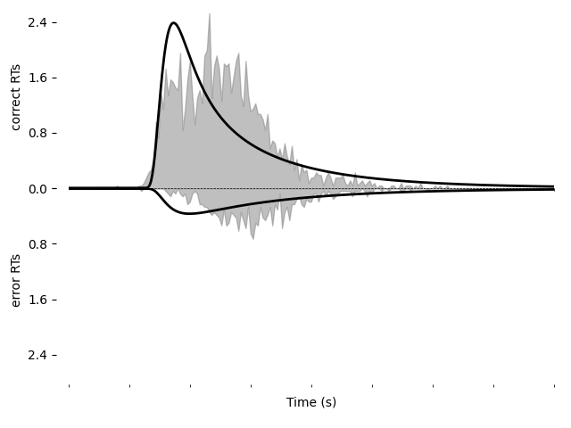
This model does not seem to fit the data very well.

We can alternatively explore this with the PyDDM’s model GUI:

# pyddm.plot.model_gui(m) # ...or...
pyddm.plot.model_gui_jupyter(m, sample=roitman_sample)

In addition to viewing the RT distributions, we can also use the model GUI to view the psychometric and chronometric functions.

# pyddm.plot.model_gui(m, sample=roitman_sample, plot=pyddm.plot_psychometric('coh'))
# pyddm.plot.model_gui(m, sample=roitman_sample, plot=pyddm.plot_chronometric('coh'))
# ...or...
pyddm.plot.model_gui_jupyter(m, sample=roitman_sample, plot=pyddm.plot.plot_psychometric('coh'))
pyddm.plot.model_gui_jupyter(m, sample=roitman_sample, plot=pyddm.plot.plot_chronometric('coh'))

See Model GUI for more info.

Download this full example

Improving the fit

Let’s see if we can improve the fit by including additional GDDM model components. We will include exponentially collapsing bounds and use a leaky or unstable integrator instead of a perfect integrator. We can implement these as we did above.

model_leak = pyddm.gddm(
    drift=lambda driftcoh,leak,coh,x : driftcoh*coh - leak*x,
    bound=lambda bound_base,invtau,t : bound_base * np.exp(-t*invtau),
    nondecision="ndtime",
    parameters={"driftcoh": (-20,20),
                "leak": (-5, 5),
                "bound_base": (.5, 10),
                "ndtime": (0, .5),
                "invtau": (.1, 10)},
    conditions=["coh"])

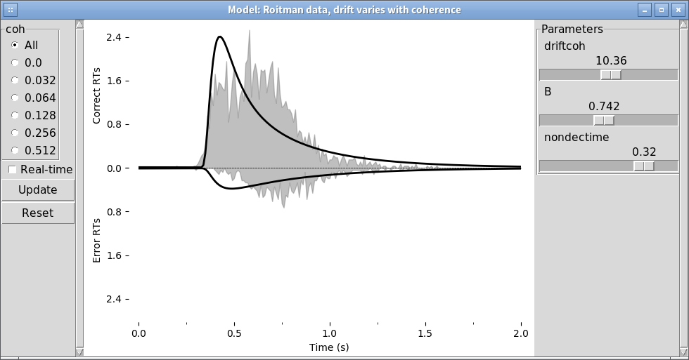
Before fitting this model, let’s look at it in the model GUI:

pyddm.plot.model_gui(model_leak, sample=roitman_sample)

We can fit this and save it as an image using the following. Note that this may take a while (several minutes) due to the increased number of parameters and because the earlier examples were able to use the analytical solver but the present example must use backward Euler. For all coherences, the fit is:

# Fit, plot, and show the result
model_leak.fit(sample=roitman_sample, verbose=False)
pyddm.plot.plot_fit_diagnostics(model=model_leak, sample=roitman_sample)
plt.savefig("leak-collapse-fit.png")
model_leak.show()

This gives the following model:

Model information:
Choices: 'correct' (upper boundary), 'error' (lower boundary)
Drift component DriftEasy:
    easy_drift
    Fitted parameters:
    - driftcoh: 9.649262
    - leak: 0.253203
Noise component NoiseConstant:
    constant
    Fixed parameters:
    - noise: 1.000000
Bound component BoundEasy:
    easy_bound
    Fitted parameters:
    - bound_base: 2.270000
    - invtau: 2.124669
IC component ICPointRatio:
    An arbitrary starting point expressed as a proportion of the distance between the bounds.
    Fixed parameters:
    - x0: 0.000000
Overlay component OverlayChain:
    Overlay component OverlayNonDecision:
        Add a non-decision by shifting the histogram
        Fitted parameters:
        - nondectime: 0.170556
    Overlay component OverlayUniformMixture:
        Uniform distribution mixture model
        Fixed parameters:
        - umixturecoef: 0.020000
Fit information:
    Loss function: Negative log likelihood
    Loss function value: -326.5744733973074
    Fitting method: differential_evolution
    Solver: auto
    Other properties:
        - nparams: 5
        - samplesize: 2611
        - mess: ''

Like before, we can still use the model GUI to visualize the RT distribution or the psychometrics/chronometric function.

Going further

In this tutorial, we have only just scratched the surface of what is possible in PyDDM. See the PyDDM Cookbook for more examples, or the API Documentation to for more details on the functions and classes used in this tutorial.

Summary

PyDDM can simulate models and generate artificial data, or it can fit models to data. Below are high-level overviews for how to accomplish each.

To simulate models and generate artificial data:

1. Define a model using gddm() or the object-oriented API. Here, we focused on gddm(). Models may depend on parameters, conditions, time, and space.

2. View your model in the model GUI to make sure it behaves the way you expect.

3. Simulate the model using Model.solve() to generate a Solution. If you have multiple conditions, you must run Model.solve() separately for each set of conditions and generate a separate Solution for each.

4. Run Solution.sample() for the Solution to generate a Sample. If you have more than one Solution (for multiple task conditions), you will need to generate a Sample for each. These can be added together with the “+” operator to form one single Sample.

To fit a model to data:

1. Define a model with at least one free parameter, using gddm() or the object-oriented API. Here, we focused on gddm(). Models may depend on parameters, conditions, time, and space.

2. Create a Sample, either using from_pandas_dataframe() or from_numpy_array(). Ensure that the conditions used in the model are present in the data.

3. Visualize your model using the model GUI to ensure it has the behavior you expect. You may need to pass the Sample you plan to fit, or else the “conditions” variable, to the model GUI function.

4. Run Model.fit() on the model and the sample. Optionally specify a loss function other than the default (negative log likelihood). After fitting, the the model will have all of its parameters specified as the fitted values.

5. View the output by calling Model.show() and the model GUI on the model. The value of the loss function is accessible via Model.get_fit_result() and the parameters via Model.parameters().