Object-oriented interface tutorial
There are two ways of interacting with PyDDM: the gddm() function, and
the Object Oriented API. gddm() is much simpler, but is not compatible
with some specialized models. The object oriented API allows you to access the
full power of PyDDM in these edge cases.
Please read the Quick Start Guide, for building models with gddm(),
before this tutorial.
Hello, world!
The object-oriented “Hello World” is almost the same as that for gddm().
The only difference is the use of Model instead of gddm().
Model will be used extensively in the rest of this tutorial.
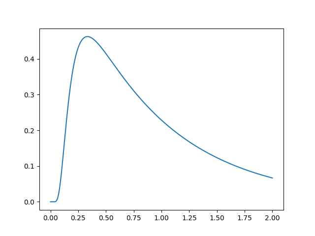
import matplotlib.pyplot as plt
from pyddm import Model
m = Model()
s = m.solve()
plt.plot(s.t_domain, s.pdf("correct"))
plt.savefig("helloworld.png")
plt.show()
Simple example
Let’s use the object-oriented API to simulate a simple DDM with constant drift. First, it shows how to build a model and then uses it to generate artificial data. After the artificial data has been generated, it fits a new model to these data and shows that the parameters are similar.
Model is the object which represents a DDM. Its default
behavior can be changed through individual model components which can be
mixed and matched.
Driftspecifies the drift rate. In GDDMs, this may change over time or across spatial positions. It defaults to a constant drift of zero.Noisespecifies the standard deviation of the noise. Most DDMs fix this to a constant, such as 0.1 or 1. However, in GDDMs, it may also change over time or across spatial positions. In PyDDM, it defaults to a constant of 1.0.Boundspecifies the shape of the boundaries which terminate the decision process. In traditional DDMs, this will be a constant, often fit to the data. However, in GDDMs, it may also increase or decrease in time. It defaults to a constant value of 1.0.InitialCondition, also known as starting point, may be a single point or a distribution of starting points. In PyDDM, it defaults to a single point centered between the bounds.Overlayallows specifying many things, such as the non-decision time. It also allows specifying mixture models when performing likelihood fitting. In general, it allows the distribution of RTs to be modified after the end of the simulation. It defaults to no no overlay, i.e., no non-decision time and no mixture model. This encapsulates both “nondecision” and “mixture_coef” fromgddm().
Each of these model components may take parameters which are (usually) unique to
that specific model component. These are specified by the model component. For
instance, the DriftConstant class takes the “drift” parameter, which
should be passed to the constructor. Similarly, NoiseConstant takes
the parameter “noise” to determine the standard deviation of the drift process,
and OverlayNonDecision takes “nondectime”, the non-decision time
(efferent/afferent/apparatus delay) in seconds. Some model components, such as
ICPointSourceCenter which represents a starting point initial
condition directly in between the bounds, does not take any parameters.
For example, the following is a DDM with drift 2.2, noise 1.5, bound
1.1, and a 100ms non-decision time. It is simulated for 2 seconds
(T_dur) with reasonable timestep and grid size (dt and
dx). Once we define the model, the solve() function
runs the simulation. This model can be described as shown below:
from pyddm import Model
from pyddm.models import DriftConstant, NoiseConstant, BoundConstant, OverlayNonDecision, ICPointSourceCenter
from pyddm.functions import display_model

model = Model(name='Simple model',
              drift=DriftConstant(drift=2.2),
              noise=NoiseConstant(noise=1.5),
              bound=BoundConstant(B=1.1),
              overlay=OverlayNonDecision(nondectime=.1),
              dx=.001, dt=.01, T_dur=2)
display_model(model)
sol = model.solve()
Solution objects represent the probability distribution functions over time for
choices associated with upper and lower bound crossings. By default, this is
“correct” and “error” responses, respectively. As before, we can generate
psuedo-data from this solved model with the sample()
function:
samp = sol.sample(1000)
To fit the outputs, we first create a model with special Fittable
objects in all the parameters we would like to fit. We specify the range of
each of these objects as a hint to the optimizer; this is mandatory for some but
not all optimization methods. Then, we run the Model.fit() function,
which will convert the Fittable objects to Fitted objects
and find a value for each which collectively minimizes the objective function.
Here, we use the same model as above, since we know the form the model is supposed to have. We fit the model to the generated data using BIC as a loss function and differential evolution to optimize the parameters:
from pyddm import Fittable, Fitted
from pyddm.models import LossRobustBIC
model_fit = Model(name='Simple model (fitted)',
                  drift=DriftConstant(drift=Fittable(minval=0, maxval=4)),
                  noise=NoiseConstant(noise=Fittable(minval=.5, maxval=4)),
                  bound=BoundConstant(B=1.1),
                  overlay=OverlayNonDecision(nondectime=Fittable(minval=0, maxval=1)),
                  dx=.001, dt=.01, T_dur=2)

model_fit.fit(samp, fitting_method="differential_evolution",
              lossfunction=LossRobustBIC, verbose=False)

display_model(model_fit)
We can display the newly-fit parameters with the
Model.show() function:
model_fit.get_fit_result().value()
This shows that the fitted value of drift is 2.2096, which is close to the value of 2.2 we used to simulate it. Similarly, noise fits to 1.539 (compared to 1.5) and nondectime (non-decision time) to 0.1193 (compared to 0.1). The fitting algorithm is stochastic, so exact values may vary slightly:
Model Simple model (fitted) information:
Drift component DriftConstant:
    constant
    Fitted parameters:
    - drift: 2.209644
Noise component NoiseConstant:
    constant
    Fitted parameters:
    - noise: 1.538976
Bound component BoundConstant:
    constant
    Fixed parameters:
    - B: 1.100000
IC component ICPointSourceCenter:
    point_source_center
    (No parameters)
Overlay component OverlayNonDecision:
    Add a non-decision by shifting the histogram
    Fitted parameters:
    - nondectime: 0.119300
Fit information:
    Loss function: BIC
    Loss function value: 562.1805934500456
    Fitting method: differential_evolution
    Solver: auto
    Other properties:
        - nparams: 3
        - samplesize: 1000
        - mess: ''
Note that Fittable objects are a subclass of
Fitted objects, except they don’t have a value.
These models function the same way as those created by gddm(). The only
difference between these two interfaces is the way the models are
constructed. Everything you do with the model after creating it, including the
use of Sample and Solution objects, is identical. Therefore, we will focus on
model construction for the rest of this tutorial.
Working with data
(View a shortened interactive version of this tutorial.)
We load the data the same way we did in the quickstart tutorial.
from pyddm import Sample
import pandas
with open("roitman_rts.csv", "r") as f:
    df_rt = pandas.read_csv(f)

df_rt = df_rt[df_rt["monkey"] == 1] # Only monkey 1

# Remove short and long RTs, as in 10.1523/JNEUROSCI.4684-04.2005.
# This is not strictly necessary, but is performed here for
# compatibility with this study.
df_rt = df_rt[df_rt["rt"] > .1] # Remove trials less than 100ms
df_rt = df_rt[df_rt["rt"] < 1.65] # Remove trials greater than 1650ms

# Create a sample object from our data.  This is the standard input
# format for fitting procedures.  Since RT and correct/error are
# both mandatory columns, their names are specified by command line
# arguments.
roitman_sample = Sample.from_pandas_dataframe(df_rt, rt_column_name="rt", choice_column_name="correct")
Now that we have loaded these data, we can fit a model to them. First we will fit a DDM, and then we will fit a GDDM.
First, we want to let the drift rate vary with the coherence. To do
so, we must subclass Drift. Each subclass must contain a name
(a short description of how drift varies), required parameters (a list of
the parameters that must be passed when we initialize our subclass,
i.e. parameters which are passed to the constructor), and required
conditions (a list of conditions that must be present in any data when
we fit data to the model). We can easily define a model that fits our
needs:
import pyddm as ddm
class DriftCoherence(ddm.models.Drift):
    name = "Drift depends linearly on coherence"
    required_parameters = ["driftcoh"] # <-- Parameters we want to include in the model
    required_conditions = ["coh"] # <-- Task parameters ("conditions"). Should be the same name as in the sample.

    # We must always define the get_drift function, which is used to compute the instantaneous value of drift.
    def get_drift(self, conditions, **kwargs):
        return self.driftcoh * conditions['coh']
Because we are fitting with likelihood, we must include a baseline
lapse rate to avoid taking the log of 0. Traditionally this is
implemented with a uniform distribution, but PyDDM can also use an
exponential distribution using
OverlayPoissonMixture (representing a
Poisson process lapse rate), as we use here. However, since we also
want a non-decision time, we need to use two Overlay objects. To
accomplish this, we can use an OverlayChain
object. Then, we can construct a model which uses this and fit the
data to the model:
from pyddm import Model, Fittable
from pyddm.functions import display_model
from pyddm.models import NoiseConstant, BoundConstant, OverlayChain, OverlayNonDecision, OverlayPoissonMixture
model_rs = Model(name='Roitman data, drift varies with coherence',
                 drift=DriftCoherence(driftcoh=Fittable(minval=0, maxval=20)),
                 noise=NoiseConstant(noise=1),
                 bound=BoundConstant(B=Fittable(minval=.1, maxval=1.5)),
                 # Since we can only have one overlay, we use
                 # OverlayChain to string together multiple overlays.
                 # They are applied sequentially in order.  OverlayNonDecision
                 # implements a non-decision time by shifting the
                 # resulting distribution of response times by
                 # `nondectime` seconds.
                 overlay=OverlayChain(overlays=[OverlayNonDecision(nondectime=Fittable(minval=0, maxval=.4)),
                                                OverlayPoissonMixture(pmixturecoef=.02,
                                                                      rate=1)]),
                 dx=.001, dt=.01, T_dur=2)

# Fitting this will also be fast because PyDDM can automatically
# determine that DriftCoherence will allow an analytical solution.
model_rs = model_rs.fit(sample=roitman_sample, verbose=False)
Finally, we can display the fit parameters with the following command:
display_model(model_rs)
This gives the following output (which may vary slightly, since the fitting algorithm is stochastic):
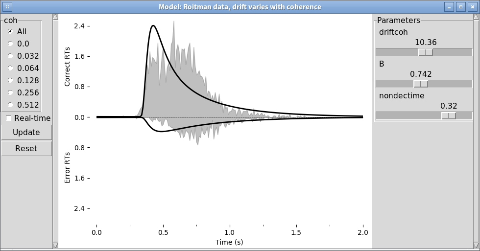
Model Roitman data, drift varies with coherence information:
Drift component DriftCoherence:
    Drift depends linearly on coherence
    Fitted parameters:
    - driftcoh: 10.388292
Noise component NoiseConstant:
    constant
    Fixed parameters:
    - noise: 1.000000
Bound component BoundConstant:
    constant
    Fitted parameters:
    - B: 0.744209
IC component ICPointSourceCenter:
    point_source_center
    (No parameters)
Overlay component OverlayChain:
    Overlay component OverlayNonDecision:
        Add a non-decision by shifting the histogram
        Fitted parameters:
        - nondectime: 0.312433
    Overlay component OverlayPoissonMixture:
        Poisson distribution mixture model (lapse rate)
        Fixed parameters:
        - pmixturecoef: 0.020000
        - rate: 1.000000
Fit information:
    Loss function: Negative log likelihood
    Loss function value: 199.3406727870083
    Fitting method: differential_evolution
    Solver: auto
    Other properties:
        - nparams: 3
        - samplesize: 2611
        - mess: ''
Or, to access them within Python instead of printing them,
model_rs.parameters()
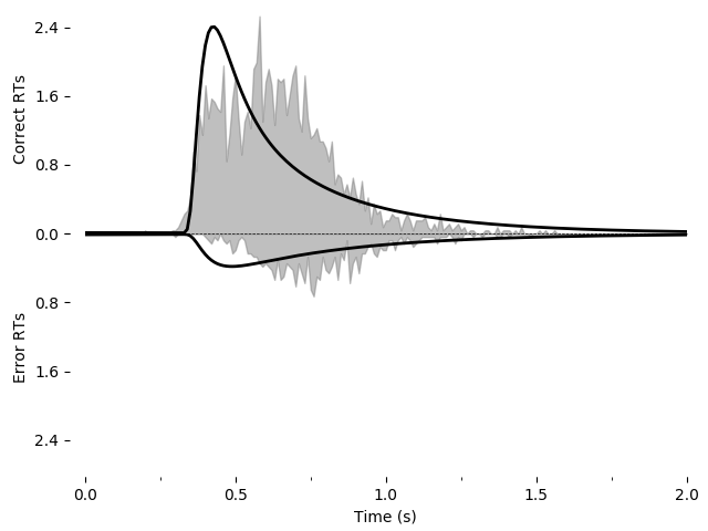
As before, we can graphically evaluate the quality of the fit. We can plot and save a graph:
import pyddm.plot
import matplotlib.pyplot as plt
pyddm.plot.plot_fit_diagnostics(model=model_rs, sample=roitman_sample)
plt.savefig("roitman-fit-oo.png")
plt.show()
We can also explore this with the PyDDM’s model GUI:
pyddm.plot.model_gui(model=model_rs, sample=roitman_sample)
Improving the fit
As before, let’s improve the fit by including additional model components. We will include exponentially collapsing bounds and use a leaky or unstable integrator instead of a perfect integrator.
To use a coherence-dependent leaky or unstable integrator, we can
build a drift model which incorporates the position of the decision
variable to either increase or decrease drift rate. This can be
accomplished by making get_drift depend on the argument x.
class DriftCoherenceLeak(ddm.models.Drift):
    name = "Leaky drift depends linearly on coherence"
    required_parameters = ["driftcoh", "leak"] # <-- Parameters we want to include in the model
    required_conditions = ["coh"] # <-- Task parameters ("conditions"). Should be the same name as in the sample.

    # We must always define the get_drift function, which is used to compute the instantaneous value of drift.
    def get_drift(self, x, conditions, **kwargs):
        return self.driftcoh * conditions['coh'] + self.leak * x
Collapsing bounds are already included in PyDDM, and can be accessed
with BoundCollapsingExponential.
Thus, the full model definition is
from pyddm.models import BoundCollapsingExponential
model_leak = Model(name='Roitman data, leaky drift varies with coherence',
                   drift=DriftCoherenceLeak(driftcoh=Fittable(minval=0, maxval=20),
                                            leak=Fittable(minval=-10, maxval=10)),
                   noise=NoiseConstant(noise=1),
                   bound=BoundCollapsingExponential(B=Fittable(minval=0.5, maxval=3),
                                                    tau=Fittable(minval=.0001, maxval=5)),
                   # Since we can only have one overlay, we use
                   # OverlayChain to string together multiple overlays.
                   # They are applied sequentially in order.  OverlayDelay
                   # implements a non-decision time by shifting the
                   # resulting distribution of response times by
                   # `delaytime` seconds.
                   overlay=OverlayChain(overlays=[OverlayNonDecision(nondectime=Fittable(minval=0, maxval=.4)),
                                                  OverlayPoissonMixture(pmixturecoef=.02,
                                                                        rate=1)]),
                   dx=.01, dt=.01, T_dur=2)
Before fitting this model, let’s look at it in the model GUI:
from pyddm.plot import model_gui
model_gui(model_leak, sample=roitman_sample)
Again, we can fit this and save it as an image using the following:
model_leak.fit(sample=roitman_sample, verbose=False)
pyddm.plot.plot_fit_diagnostics(model=model_leak, sample=roitman_sample)
plt.savefig("leak-collapse-fit-oo.png")
Going further
Just as we created DriftCoherence above (by inheriting from Drift)
to modify the drift rate based on coherence, we can modify other
portions of the model. See PyDDM Cookbook for more examples. Also
see the API Documentation for more specific details about overloading
classes.
Summary
PyDDM can simulate models and generate artificial data, or it can fit them to data. Below are high-level overviews for how to accomplish each.
To define models in the object-oriented API:
Optionally, define unique components of your model. Models are modular, and allow specifying a dynamic drift rate, noise level, diffusion bounds, starting position of the integrator, or post-simulation modifications to the RT histogram. Many common models for these are included by default, but for advance functionality you may need to subclass
Drift,Noise,Bound,InitialCondition, orOverlay. These model components may depend on “conditions”, i.e. prespecified values associated with the behavioral task which change from trial to trial (e.g. stimulus coherence), or “parameters”, i.e. values which apply to all trials and should be fit to the subject.Define a model. Models are represented by creating an instance of the
Modelclass, and specifying the model components to use for it. These model component can either be the model components included in PyDDM or ones you created in step 1. Parameters for the model components must either be specified expicitly or else set to aFittableinstance, for example “Fittable(minval=0, maxval=1)”.Simulate and fit the model, as with
gddm().